Google Sheets provides a variety of functions to perform rounding operations on numbers, INT Function being one of them.
Using INT Function you can very easily round down decimals to nearest Integer values. Lets cover all the necessary components and gain complete understanding of dynamics of INT Function.
Table of Contents
Purpose of INT Function
INT Function rounds down the number to nearest integer that is less than or equal to it.
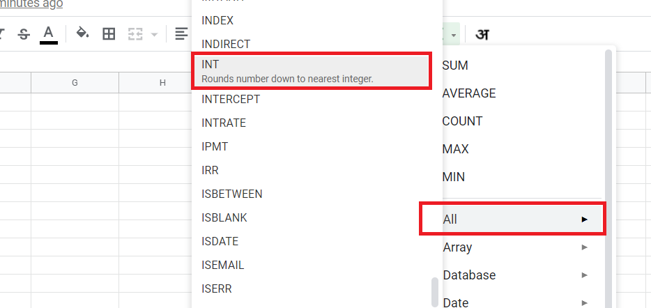
To use it simply type “=INT(” place the number within and close the bracket. Another ways is to click on the function dropdown in the Toolbar.

Syntax and Parameter Definition
=INT(value)- value: Any static number/cell reference which needs to be rounded down to nearest integer.
Note:
- INT Function only accepts numerical input.
- Any form of non-numerical input(like “abc”, “xyz” etc) will result in an “#VALUE!” error.
- INT is fundamentally different from both CEIL(significance of -1) and ROUNDDOWN(places is set to zero)
- It’s similar to FLOOR function with a factor of 1 {=FLOOR ( Value ,1)}.
Expected Output
INT Function returns the nearest integer(as a whole number), less than or equal to the supplied value input. Below are some examples to help us understand this concept better.

An important point to notice here is the treatment of negative decimal numbers. As visible the negtive decimal numbers are rounded up to higher level of integer (-10.2 becomes -11) in absolute terms. But yes -11 is less than -10.2, hence we are still very much consistent with then definition of INT function here.
Visual Demonstration of INT
Before we end here is a simple visual demonstration of INT Function

That’s it on this topic. Keep browsing SheetsInfo for more such useful information 🙂


