Dropdown lists is a very handy tool to promote data standardization and provide ease of input to Google Sheet users. There are multiple ways to create a dropdown list which we have covered here.
In this tutorial we will understand the process of adding a cell color depending on the option selected in the dropdown list. We will be using conditional ‘ formatting to achieve this objective.

Table of Contents
Sample Google Sheet File
In this tutorial we will be using the below Google Sheet Document to work. Feel free to create a copy for yourself.
Creating a Dropdown Lists
To those who are new to the concept of Data Validation and Dropdown Lists you can get visit below links.
Or, a quick recap below would also be useful to juggle the memory.
Creating Dropdown Sheet using List of Items Option
Creating Dropdown Cells using Cell Range Option


Adding Conditional Formatting to Cell
To add color to Dropdown lists follow the below steps:-
- Create a Dropdown Lists in a cell
- Select the cell , Goto Format -> Conditional Formatting
- Select the Rule, Add the value & decide the formatting
- Repeat step 3 for all possible dropdown options
Lets deep-dive into individual steps in more detail.
Step 1: Create a Dropdown list
Follow the instruction in previous steps to create a dropdown list. For the purpose of this exercise we shall create a simple dropdown list with three options, “Yes”, “No”, “Maybe”

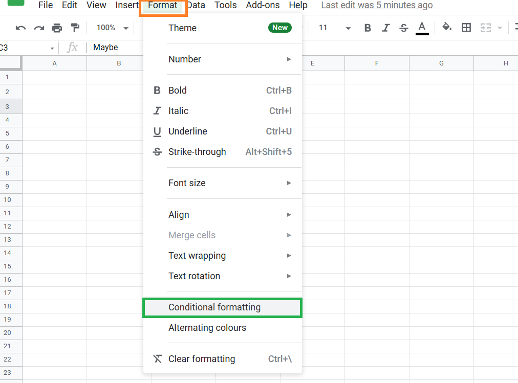
Step 2: Open conditional Formatting Option
Goto Format -> Conditional Formatting
Step 3: Add Conditional Formatting Rules
Lets say, I am looking for the below formatting against the dropdown optional selected
YES -> Green
NO -> Red
MAYBE -> Yellow
Lets start with the implementing the first rule.
In the “Format Cells if” select “Text is Exactly” and then enter “Yes”. Lastly goto Formatting style and select Green fill. In a similar way you can workout for the other two options as well.


Once the above steps are completed, we would now be able to select dropdown options with automatic color fill basis selection.

That’s it on this topic. If you face any issues in implementing the above methods then leave a comment down below. Keep browsing SheetsInfo for more such useful information 🙂