CEIL Function belongs to the family of Mathematical functions in Google Sheet used for rounding numbers.
CEILING Function stands apart from other sister functions like Round/INT/TRUNCT etc since it lets you round a number to nearest multiple of a specified significance. Does sound a bit tricky right? Not anymore once you go through this article.
Lets cover all the necessary components and gain complete understanding of dynamics of CEIL Function.
Table of Contents
Purpose of CEIL Function
Google defines TRUNC Function as “Truncates a number to a certain number of significant digits by omitting less significant digits“. And this is exactly what it does as well.
To use it simply type “=TRUNC(” place the number within and close the bracket. Another ways is to click on the function dropdown in the Toolbar.
Syntax and Parameter Definition
= CEILING(value, [factor])- value: The number you want to round to nearest integer multiple of factor
- [places]: the number to whose multiple the value will be rounded.
Note:
- CEILING Function only accepts numerical input.
- Any form of non-numerical input(like “abc”, “xyz” etc) will result in an “#VALUE!” error.
- [factor] is an optional input. 1 is it’s default value.
Expected Output with Examples
Google describes Ceiling Function usage as ” rounds a number up to the nearest integer multiple of specified significance”.
In simpler words, CEILING Function will look for next highest number to Value, whose significance is an multiple of factor specified in the formula.
Surely, we need more than just the above statement to understand usage of Ceiling Function. Let’s look some cases to understand better.
Simplest Case
Below is a text book case of how CEILING Function works.

In the first case, factor is 10 and next highest number to 253.212 which is a multiple of 10 is 260. In the sixth case there the closest number to 253.212 of one decimal place and a multiple of 0.5 is 253.5. Similarly, you can easily interpret output for other cases as well.
Working with Decimals
In the below example, we are only working with decimal factors and dealing with different level of significant digits.
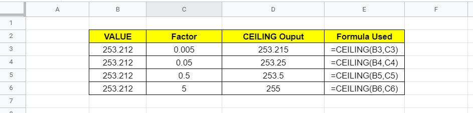
As we can see the number of significance digits in the output is directly controlled by factor we had. The output is greater the Value as expected.
Positive and Negative Numbers
Negative numbers are fundamentally treated in a similar way while working with CEILING Function. However, the results as we can see below are slightly different.

The above different can be solely attributes to the fact that for negative numbers say a -250 > -253.212. This is the main reason for the difference we are seeing.
Visual Demonstration of CEIL
Before we end here is a simple visual demonstration of CEIL Function.
That’s it on this topic. Keep browsing SheetsInfo for more such useful information 🙂