ROUNDDOWN Function belongs to the family of Mathematical functions in Google Sheet used for rounding numbers.
It’s very similar to ROUND Function, just with the difference that it will always Round-down. Let’s go through the salient features of ROUNDDOWN Function in this tutorial.
Table of Contents
Purpose of ROUNDDOWN Function
As you would have guessed, it helps us to round numbers and retain decimals upto a specified decimal place.
One important callout for ROUNDDOWN is that it always picks the lower value while rounding off. This means
ROUNDUP(32.76,1) equals 32.7and
FLOOR(32.73, 1) equals 32.7Before jumping onto examples let’s understand the syntax of ROUNDUP.
Syntax and Parameter Definition
= ROUNDdOWN(value, [places])- value: The number you want to round
- [places]: The number of decimal digits you want to round the ‘value’ to.
Note:
- Value can take only numerical input
- Any form of non-numerical input(like “abc”, “xyz” etc) for value will result in an “#VALUE!” error.
- [places] is an optional input. 0 is it’s default value.
- [places] should be an integer either positive or negative.
- You can directly add static values or cell references for both value and [places]
Expected Output, logic behind it and Examples
ROUNDDOWN function follows a very simple logic to operate.
Say, you want to round up to 2 decimal places. ROUNDDOWN will retain the number upto two decimal place. What is present in the third decimal place will have no effect on ROUNDDOWN Operation.
Simplest Case – ROUNDDOWN Function
Below shown example is a very simple example of how ROUNDDOWN works and where is it different from ROUND Function.
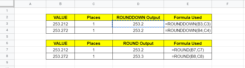
As you may have observed in both the cases ROUNDDOWN Function returns an output which is nothing but retaining the once decimal place and discarding the rest.
More Examples – ROUNDDOWN Function
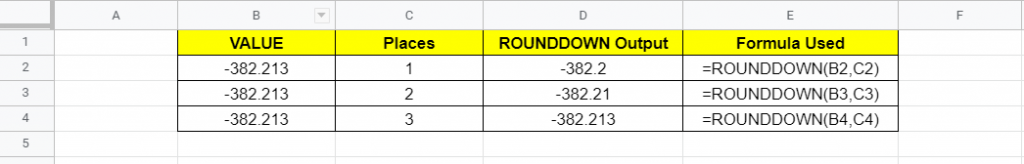
In the below example we have taken the liberty to play around with Places. Let’s discuss the insights we can derive from the below.

In, the first three case we have varied the [places] keeping Value same. The outputs are pretty self explanatory as well. In all cases ROUNDDOWN has retained the number of decimal places it was specificed.
In the last two cases, we kept places as 0/missing. Not surprisingly, the results are same as default value of [places] if not supplied is 0. Having [places] as 0, gives an indication to ROUNDDOWN that we don’t need any decimal value, hence the result it a whole number.
Working with Negative ‘Value’
We used the same cases from last example, just added a minus sign before it. Clearly, there’s no effect to working of Roundup Function. The output we got last time is intact this time as well.
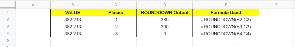
Working with Negative ‘Places’
Having Negative value in ‘Places’ results in rounding down to nearest Ten’s/Hundred’s/Thousand’s depending on the value of Places(-1/-2/-3 and so on)
Visual Demo of ROUNDUP Function
Before we end here is a sample visual demonstration of ROUNDUP Function in action.
That’s it on this topic. Keep browsing SheetsInfo for more such useful information 🙂