Conditional counts are frequently required whenever you are trying to draw insights from a big dataset. One such instance is when you want to count cell any text/specific text across a group of cells.
While you can use Google Sheet Filters to easily get it done, there are also smart ways to getting this done using formula.
In this tutorial, we’ll cover all these questions in detail. Stay Tuned.
Table of Contents
Count Cells Containing any Text in Google Sheet
If you are just looking to count cells which contain any kind of text entries and ignore the rest then this section is for you.
To get this done, we will be using COUNTIF Function along with Wildcard Character(*).
Say, you have the below data range, from which you want to count only cells containing any text(highlighted ones).
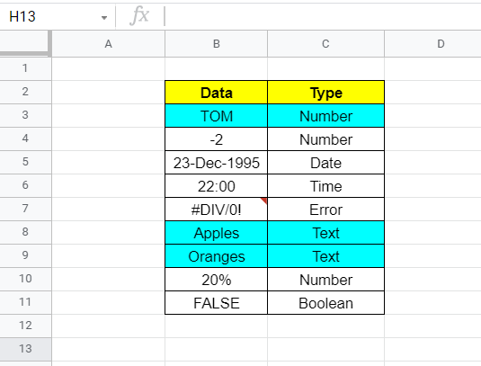
We will use the below formula to get the results:
=COUNTIF(B3:B11,"*")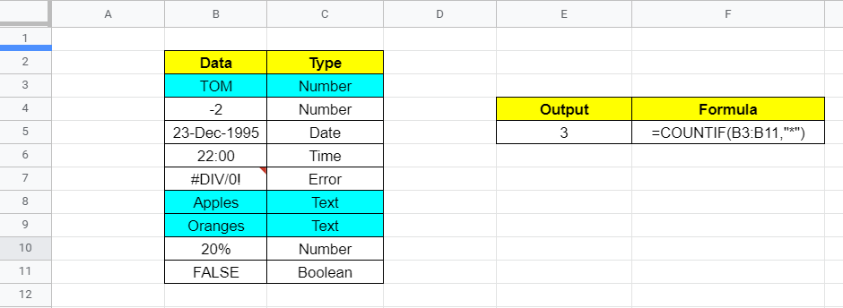
As you can see above, we exactly got the result(3) we wanted. Let’s now breakdown the formula to understand what’s going on behind the curtains.
Firstly, COUNTIF Function is meant to return conditional counts. It takes in a range(B3:B11) and a criterion(“*”). Only cells in the range that fullfill/pass the criterion will be counted.
In above case choice of range is a no-brainer. Criterion is “*”, which is nothing but a wildcard character. * simply represents a group of characters. Hence, all cell which had any group of characters were counted.
Count Cells Containing Specific Text in Google Sheet
Taking a step forward lets try to now count cells only containing a specific text(wholly/partially).
In the below example we want to find all cells containing “Apple”. We have again called out COUNTIF to the rescue. This time the criterion will be “Apple” as we are just looking to count cells containing “Apple”.

Note: The text matching is not case-sensitive, hence an Apple, apple or APPLE would give the same results.
So what happens, when you need a count, but you want to just check a partial match of a text.
Say, in below example you want to count all entries containing apple(highlighted ones).
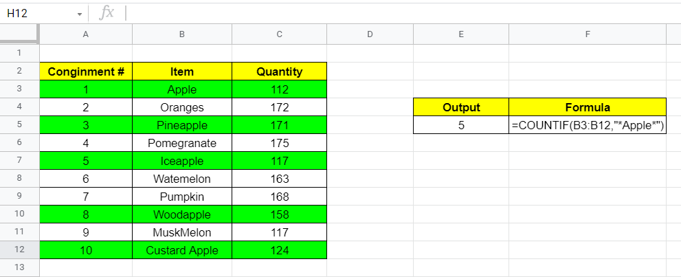
As you can see, we made a minor modification to the previous formula. Now the critetion is “*Apple*”. Appending the wildcard character asterisk(*), means that any number of characters can come before/after the word “Apple”.
This effectively converts the criterion from a specific match to a partial match.
Visual Demo of using COUNTIF
Before we end the topic lets see how to implement the above solutions in action.

That’s it on this topic. Keep browsing SheetsInfo for more such useful information 😊

