When juggling with large amounts of data, the most frequent operation is creating new columns and applying custom formula’s to the entire column. Even for newbies learning this operation will prove to be a big time saver.
Fortunately, Google Sheet provides us with multiple methods to apply formulas to the entire columns(or rows). Lets cover the important ones in this Tutorial
Table of Contents
Using Mouse Controls
We can very easily apply formulas to entire columns using basic mouse controls like Double-Click and Drag & Drop.
Lets discuss both of them in details
Automatic Drag Using Double Click Method
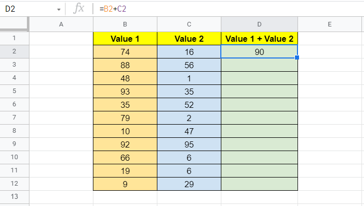
Step 1: Apply formula to the First Cell, say D2 for the example below(or any custom starting cell of your choice).

Step 2: Press Enter to realize the output.
Step 3: Move over to the right-bottom edge of the cell, over the square dot until the cursor turns into “+” shaped tool, called Fill Handle.
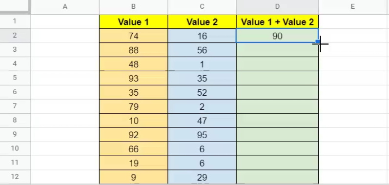
Step 3: Now Double Click over the square dot. You’ll observe that the formula gets uniformly applied till the end of the table. See final results below.

A big ‘Pro’ of using this method is that it’s easiest to execute and will give you the indented output 99% of the time. One ‘Cons’ worth highlighting is that if you have any vacant rows in between then the automatic formula application will stop over there.
In other words, we have to ensure that there are no absurd gaps in data while applying using this method.
Using Drag and Drop Method
A bit more manual than the previous method, but with slightly more control. The Steps are very similar to the previous method. Instead of double-clicking the square dot, we click and hold the mouse over the square dot. Now without releasing mouse slownly drag down and you will pbsevre the formulas getting applied to all cells beneath.
Below visual tutorial should be able to help.
Clearly, this method will only be useful while working with smaller datasets. Also, to highlight, any formatting associated with the first cell(D3 in example) will also get applied along with the formula to other cells in the column.
Using Paste-Special Method
Paste-Special always has something useful to offer. In this case, idea is to copy the cell containing the formula. Then Paste only formula part of the cell to the other cells listed below.
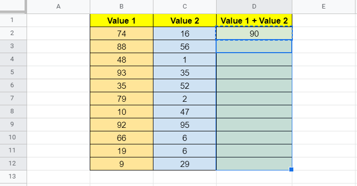
Step 1: Apply the formula to the first cell and press enter to realize the output.

Step 2: Once done Right Click and Copy cell D2 or press CTRL + C.
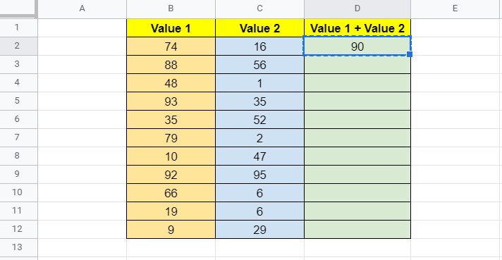
Step 2: Now select all the cells from D3 to D12. You can simply use your cursor( or press SHIFT+Down+Down… upto D12)
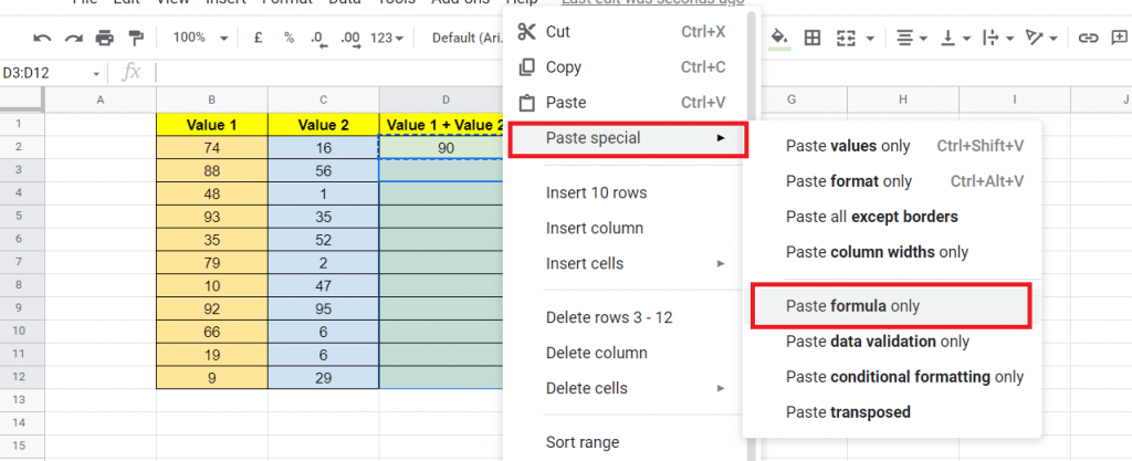
Step 3: Now Right Click -> Paste Special -> Paste Formula Only
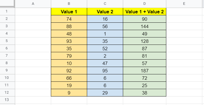
Step 4 : We get the intended results for D3:D12

Using ARRAYFORMULA Function
ArrayFormula Function is a very special function which will enable you to apply formula to just first cell, say D2 below and all the entire target array will have the formula applied.
To do this it basically requires a simple tweak to the formula we have writing generally like below.
=ARRAYFORMULA(B2:B12 + C2:C12)Something like this:

Now Press Enter and we get out desired result.

One major Cons for this method is that you cannot make changes to formula of individual cells like D5 or D7. Any change made will have to be on D2.
Using Autofill Keyboard Shortcut, CTRL+D
This is generally less talked about but once again very useful and practical method.
Step 1: Simply apply the Formula to D2. And Select all Cells from D2:D12.

Step 2: Now Press Ctrl + D from the keyboard. We Have the formula uniformly applied across all cells from D2 to D12.
That’s it on this topic. Keep browsing SheetsInfo for more such useful information 🙂