How to Multiply in Google Sheets

Fundamental mathematical operations like Addition, Subtraction, Multiplication & Division are very easy to do in Google Sheets. In this article we will focus on the use of MULTIPLY() Function and ‘*’ [Asterisk Operator] to perform Multiplication in Google Sheets.

We’ll also cover associated caveats and couple of practical examples to boost our understanding in this topic.

Using Asterisk “*” Operator

This is probably the most simplest method if you are looking forward to do a simple multiplication task in Google Sheet. You just need t type “=”followed by all the numbers you wish to multiply separated by Asterisk Operator “*”.

Syntax and Parameter Definition

= Factor1*Factor2*Factor3.....

Note:

1. You can add as many factors as you want
2. You can add static value, cell references
3. Non-numeric inputs will result in an error
4. Empty cells will be treated as a 0 while performing the multiplication operation.

Expected Output

As expected we get the final result after multiplying all the input Factors listed out in the formula. Below are couple of examples demonstrating the use of * operator in action.

It’s clear from the above example that we can have both static value and cell references as inputs. Also supplying string values will result in an error(row 5). As indicated by example in row 4 we have to be super cautious while using cell references in the formula. A missing/blank cell like C4 can render the entire calculation useless since the missing value will be treated as 0 during the calculation.

Using MULTIPLY() Function

Google Sheet offers a simple MULTIPLY Function to help with multiplication activities. You can simply type it out in the cell or use the function dropdown on the toolbar to select the option.

Syntax and Parameter Definition

=MULTIPLY(factor1, factor2)

Note:

1. You cannot enter more than 2 arguments in Multiply Function
2. You can only add scalar values(2,3,4 etc) or cell references(A1,B1 etc) as argument. Cell Ranges are cannot be used in the arguments.
3. Non-numeric inputs like characters, string etc will result in an error.

Expected Output

Multiply Function returns the output of multiplication of the two input parameters. Let’s look at a couple of examples to get a better clarity of the functioning of the MULTIPLY Function.

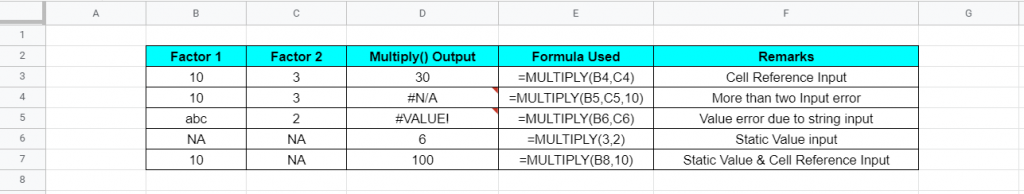
Some of the things we discussed previously are now becoming very clear. In Row 4, we supplied more than 2 inputs which resulted in a #N/A error. Similarly in Row 5. we entered a String input ‘abc’ which caused a ‘#VALUE!’ error.

In row 6 & 7 we have demonstrated as to how we can supply static values as well to the Multiply Function.

Using PRODUCT() Function

PRODUCT Function() is the enhanced version of Multiply Function and * operator. It truly helps to overcome all the limitations present in the above two methods.

To use the Product Function you can simply type “=PRODUCT(” or can use the dropdown available in the formula toolbar.

Syntax and Parameter Definition

=PRODUCT(factor1, [factor2, ...])

1. Factor1 : First number/range to be multiplied with
2. [Factor2,…]: OPTIONAL- Additional Number/Range to be used for multiplication

Note:

1. You can add as many arguments as needed
2. You can use both scalar values(2,3,4 etc), cell references(A1,B1,C1 etc) or cell ranges(A1:A10 etc) in the formula
3. Non-Numeric Inputs, Black Inputs will be ignored during calculation

Expected Output

Let’s straightaway jump to the examples to get a better understanding of the PRODUCT Function.

As you can see from above example PRODUCT Function is vastly supreoir to earlier methods. It quitely ignores empty inputs[row4] instead of treating them as 0. It also ignores non-numeric inputs while calculation[row5].

Best part is you can use a range of numbers input as well[row7] along with other static values and cell references.

Multiply Entire Column in Google Sheet

More often than not you will need Google Sheet help for completing large scale multiplication operations across multiple rows and columns. In this section we will discuss some of such examples.

OPTION 1: Drag and Drop Multiplication Formulas

Simply apply the mathematical formula for multiplication and select the square box at the edge of the cell , click and hold and drag down. Below video should help explain.

OPTION 2: Using ARRAYFORMULA Function

This is a smart way to achieve the same results as we got in OPTION 1. Simply use the below formula in cell D3. The output will be pasted over entire cell range we were looking for.

=ARRAYFORMULA(B3B24 * C3:C24)

That’s it on this topic. Keep browsing SheetsInfo for more such useful information 🙂