Freeze Row/Columns in Google Sheets

It’s fairly common to forget the mapping of row headers when scrolling through a very large spreadsheet. Hence, it’s advisable to Freeze Rows(or Columns) which you would prefer to be locked while scrolling through the sheet.

Two Ways to Freeze Rows

Freezing Rows is fairly straightforward and can be done via multiple ways in Google Sheets.

Using Menu Option

1. Open the Sheet where you would want to Freeze Rows

2. Now in Menu Bar goto View->Freeze -> 1 Row

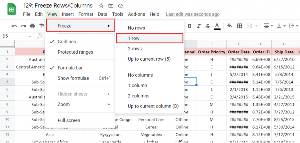
3. The First Row now gets locked. This is also evident by the bold light gray line visible below the first row.

Now, even if you scroll down the first row will be locked in one place as expected.

Using Mouse Shortcut

This is a handy method to Freeze Rows and will definitely differentiate you from the crowd. Follow the below steps apply this method:

1. Move the cursor near the boundary of first row until to observe a the arrow symbol turning to a hand shape icon
2. Click and hold when the Hand shaped icon appears and drag down

Something like this:-

Freeze Multiple Rows

At times it might make more sense to freeze multiple rows at a time as per the requirement. This is also pretty straightforward to do.

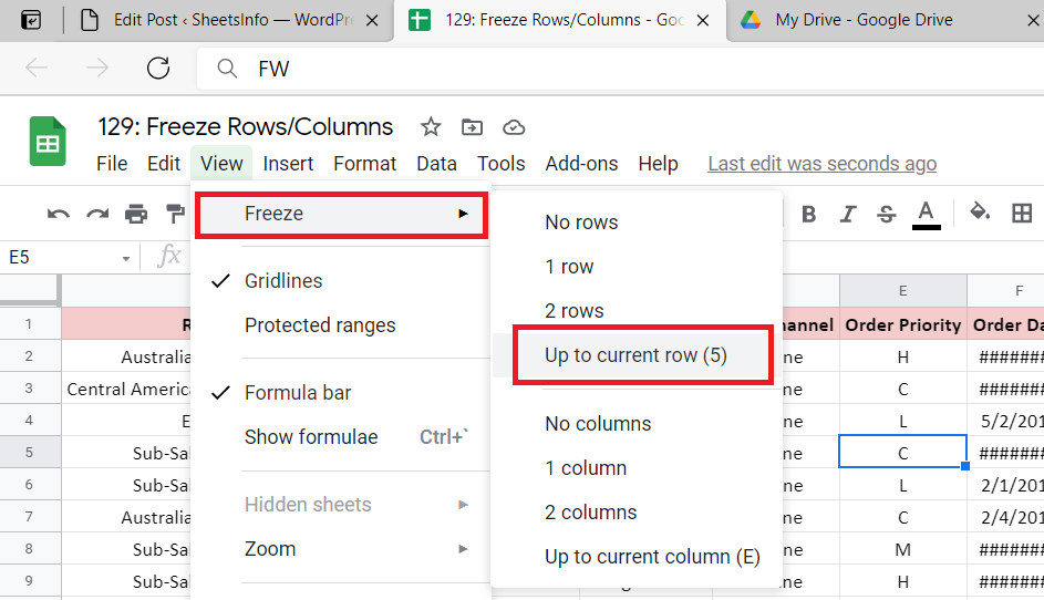
Say you need to freeze first 5 rows. Select any cell in 5th Row.

1.. Select any cell in 5th Row

2. Goto View -> Freeze -> Up to current row(5)

Alternatively, you can use the mouse shortcut to achieve the same goal.

Two Ways to Freeze Columns

We can freeze columns using very similar method as discussed above.

Using Menu Options: Follow the same approach as discussed before. Select either 1 Column/2 Column/Upto Current Column as per need.

Using Mouse Shortcut:

Unfreezing Row/Columns

Simply goto Menu -> View -> Freeze. Select both no row and no column in two iterations.

Post this operation any frozen cells will removed from the current worksheet.

Points to Note

1. Both Rows and Columns can be frozen in a Google Sheet
2. Use Menu Option View -> Freeze to apply or remove freeze setting to rows and columns
3. Changing Freeze options in one Sheet will not effect Freeze settings in another Sheet.

That’s it on this topic. Keep browsing SheetsInfo for more such useful information 🙂