COUNTIF Function helps to perform conditional counts depending on a condition. It’s a bit more advanced from the regular COUNT function in this regard and is a part of a group of similar other functions like COUNTA, COUNTIFS etc
In this tutorial we will take you through the all the important aspects of COUNTIF Function.
Table of Contents
Purpose of COUNTIF
As indicated before COUNTIF helps us to get conditional counts.
But what does the above mean? For example, say we have below range of numbers, in Google Sheet. And we want to find out number of people with a weight of over 70 kgs.

To achieve this, we can simply use the below COUNTIF Formula.
=COUNTIF(D3:D10,">70")We have detailed out more examples in subsequent sections. However, before that lets firstly let’s understand the syntax and associated constraints for COUNTIF Function in the following section.
Syntax and Parameter Definition
= COUNTIF(range, criterion)- range: It’s the group of cells(like A3:A7, B2:B10 etc) which needs to be counted, against a specific criterion.
- criterion: If the rule or condition(like “>10”, “=5”) which needs to be satisfied for count to get registered. You can include comparison operators like <, > , <=, >=, = , <>
Important Points to Note:
- Range can have number or string values. However, if Range is string then criterion must be too and vice-versa.
- Criterion must be enclosed in double quotes like “=5”, “>7” , “STAR”
- One can easily use wildcard characters like *, ~ etc while specifying the criterion for a text condition
- Both Range and Criterion can be specified with cell references like COUNTIF(B3:B7,C1)
- COUNTIF is case-insensitive while checking for text criterions
- Empty cells in the range are excluded from the count operation
Expected Output
COUNTIF returns the count of number of cells, within the specified range which fulfill the condition specified in Criterion.

The output can very well vary basis the criterion specified.
It’s important to highlight here that COUNTIF can only take one Criterion at a time. If you want the count basis multiple criterion then it’s use COUNTIFS which is a better alternative.
Hope, it was clear till here. As you can see COUNTIF is pretty easy to understand once you have understanding of the basics.
Examples
Let’s now cover some practical examples to grasp the usage of COUNTIF better. We’ll touch upon both type of cases where Criterion is number based vs text based.
Count number of times a value is <,>,=,<> in the Range
Although we have already seen comparison operators in action before, lets cover it again in a bit more detail.
We have tried to cover all the operator Criterions in the below example.


Counting Blank or non-Blank Cells in a Range
From all that we have learnt till now this should be an easy one.
To Count Blank Cells only deploy the following logic.
=COUNTIF(range,"")To Count Non-Blank Cells only deploy the following logic.
=COUNTIF(range,"<>")
Count number of times a word occurs in a range – Exact Match
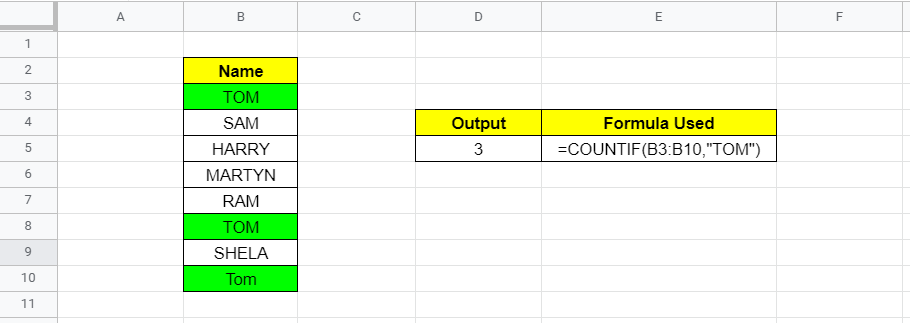
Say we want to know how many time “TOM” occurs in the range B2:B10. This can be done using the simple formula below:
=COUNTIF(B3:B10, "TOM")
Note: As evident COUNTIF doesn’t take into account upper/lower case while matching. Count is 3 including both “TOM” and “Tom”
Count Number of Times a word occurs – Partial Match
Wildcard Characters in Google Sheet can be easily used when there’s a need to create partial text match conditions.
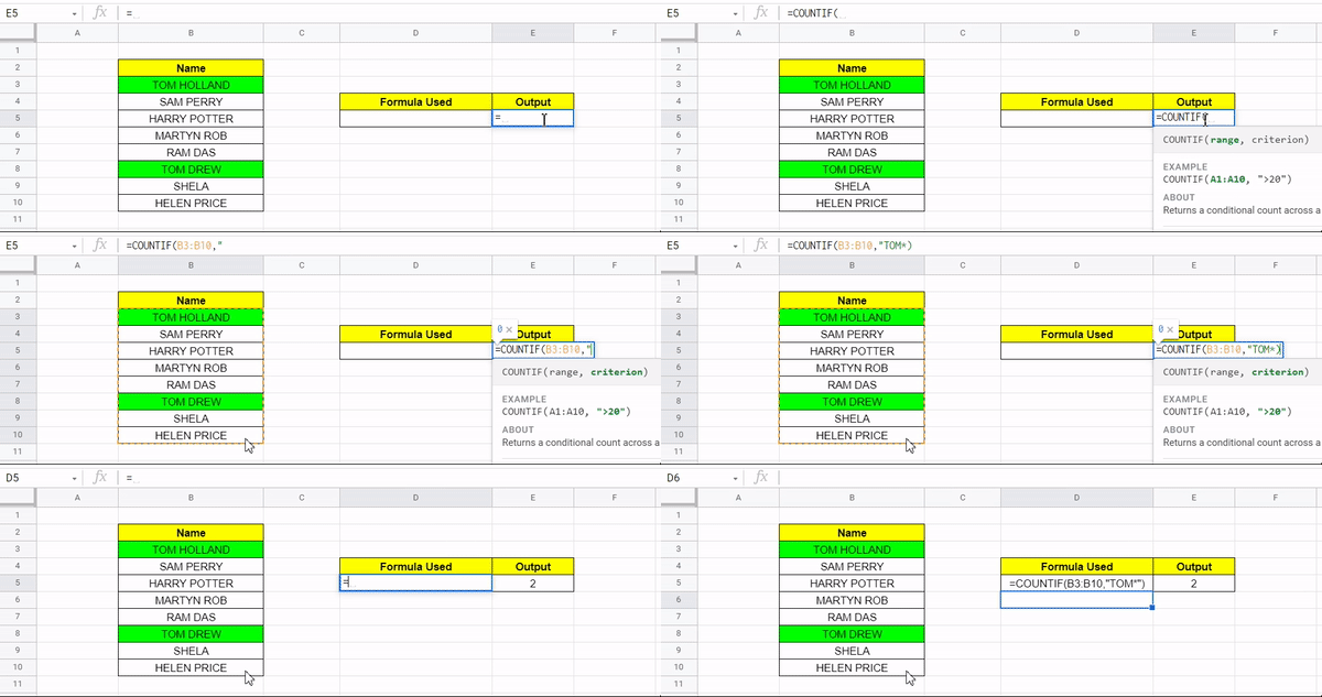
Say we want to count all cells where with Names Starting with TOM. We’ll use the Wildcard Character * to achieve this objective.
=COUNTIF(B3:B10, "TOM*")When we put a Criteria like “TOM*” , it will matching anything which starts with TOM.

Visual Demo of ROUNDUP Function
Before we end here is a sample visual demonstration of COUNTIF Function in action.

That’s it on this topic. Keep browsing SheetsInfo for more such useful information 🙂


