At numerous occasions each one of us have encountered the text spilling/trimming issues like below. Such a poor representation of data is detrimental to user experience, especially for information sensitive tasks.

In this post we will discuss about various methods of using text wrapping options provided in Google Sheets.
Table of Contents
Basic Text Wrapping in Google Sheets
This section will be relevant to most of the readers. If you are looking to apply a transformation as shown below to wrap word & fit to cell then continue reading.

Text Wrapping using Format Option
- Select Cells which you wish to wrap. Simple place your cursor over the top-left cell. Click and Hold, now drag all the way upto bottom-right.

2. Now goto Format -> Text Wrapping -> Click Wrap

3. The Selected Cells now get wrapped. We now have the full view of the text without loosing any information
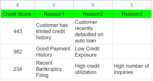
Note: Column width remains the same. Only the row height increases.
Wrap Text using Quick Access Toolbar Shortcut
Another way to get the same results is use Text Wrapping options available on the toolbar.
- Simply select the target cells and head over to the below option in the tool bar and click.

2. Now click the second button in the dropdown.

3. As expected we get the similar desired result

Wrap Text Manually
You would have already noticed by now that during wrapping operation we do not have control on how the like text gets arranged. Google Sheets does it’s best to fit as many words within the given column width before moving on to the next line.
But what if you want to customize it because the requirement is such. Manual Text Wrapping now comes to help.
Say, you have an address like below, Cell C4. If you try the methods discussed previously you get an output like C5. Good, but certainly not the most desirable. Cell C6, created using Manual Wrapping looks much more structured.

- Start by clicking the cell, in our case C6 which you would want to manually wrap. Now double click or press F2 to enter into editing mode.

2. Now move the cursor to the position post which you would like to skip to next line. For us its post ‘6/151,’.

3. Now Press Alt + Enter.

Now, repeat steps 2 & 3 unless you arrange the text in the way you want. Once done, press Enter. We get the desired output using Manual Wrapping Method.
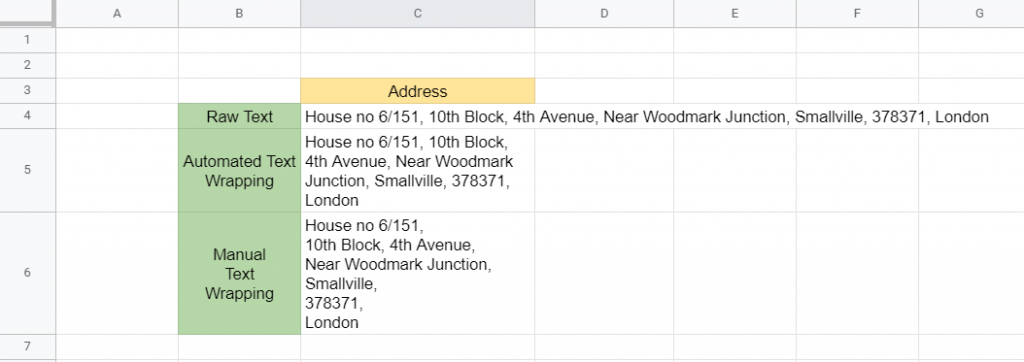
Note: This method is not scalable and would have to be applied one Cell at a time.
Text Clipping in Google Sheets
This is another Text Wrapping option which deserves a final mention before we end this post. This is the Clip Option.
So, what does Text Clipping do. It restraints text display only to current cell and doesn’t let it spill over.
B1 and B2 have the exact same text with the exception that B2 is Clipped hence there is no Spillover to C2.

- Select the Cell which you would like to Clip. In our case, this is B2.

2. On the Menu Bar goto Format -> Text Wrapping -> Clip
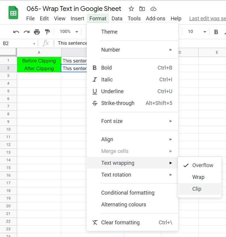
or Click the Third button in Text Wrapping Toolbar option.

3. As Expected, post Clipping the cell there is no spill-over of text in cell B2.

Unwrap Text in Google Sheet
Follow the similar steps as before and select Text Overflow to Unwrap Text in Google Sheet.
Below Clip should help with the same.

Points to Note
- Two Text Wrapping options in Google Sheets are Wrap and Clip
- Columns width remains constant in either of the Text Wrapping Option
- You can either use Tool Bar or Menu Options to apply Text Wrapping
- Manual Text Wrapping method is customizable but not scalable
That’s it on this topic. Drop a comment below in case of any questions. Keep browsing SheetsInfo for more such useful information 🙂

