Gridline happens to be the most fundamental feature of any Spreadsheet application. While, they are very essential in data visualization, sometimes we are better off without them. Hiding gridline is very simple task and very handy at times.
In this tutorial we will discuss about different methods to show or hide gridlines. Also, how can we show/hide gridlines while printing spreadsheets.
So, lets begin.
Table of Contents
Remove(or Show) all Gridlines using the Menu Option
As always, lets open a sample spreadsheet.
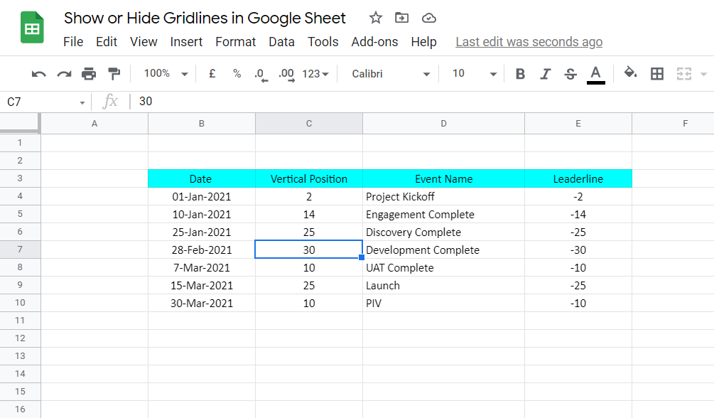
Under Menu Bar, goto View -> Gridlines and click.
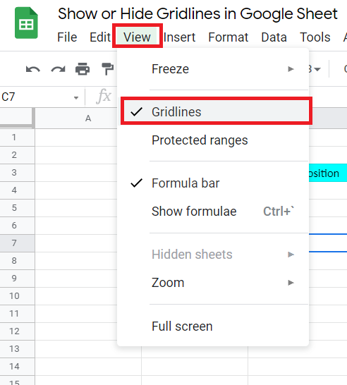
Since, we unselected Gridlines, you will observe that all the gridlines are removed.
In a similar manner, you can also Show gridlines by following the same approach. Like below:-
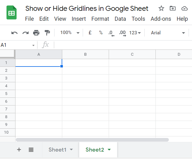
Note: This change is sheet specific. Other Sheets(like Sheet2 below) will still continue to have gridlines. To remove gridlines from Sheet2, same operation will have to be repeated.
Action on Specific Gridlines
Above mentioned approach would end up impacting all the rows and columns. However, in case you want to hide or show a specific group of cells then we will take a different approach.
Hide Specific Gridlines
There’s no direct way to “Hide Specific Gridlines” in Google Sheet. We’ll improvise to get our job done here.
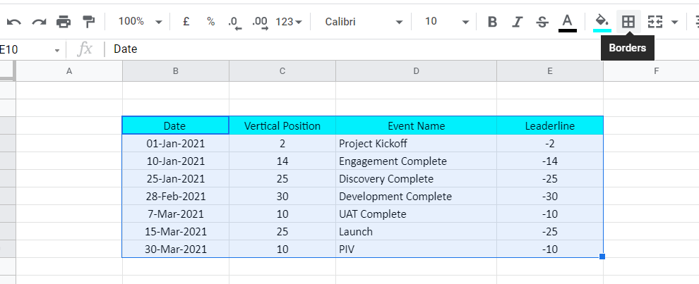
Select the group of cells where you want to hide the gridlines and goto Border icon in the quick access toolbar.
Firstly, select the color as White.
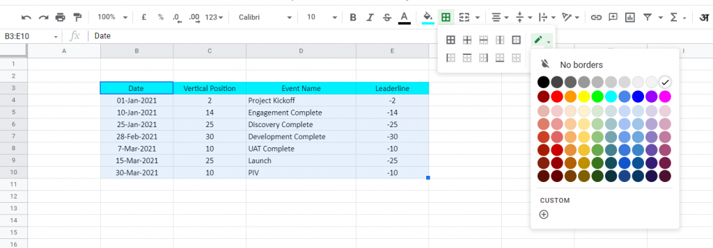
Now, Select the first option to enable “All Borders”

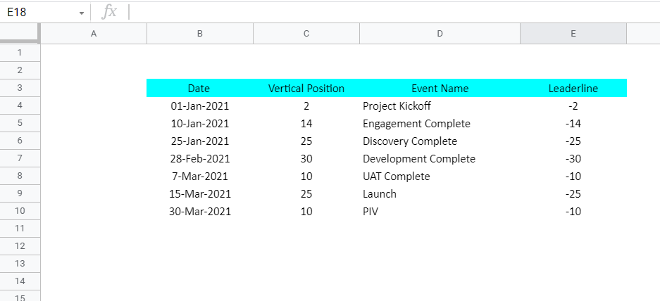
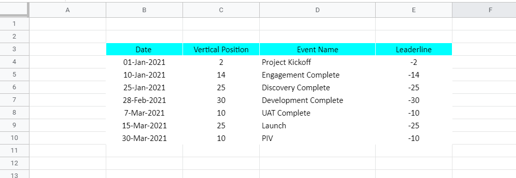
Final result. In effect, we didnt hide gridlines but simply added a border which was “white”.
Show Specific Gridlines
Once, again no direct way to do this either. This time, we hide all the gridlines first. Then we add borders to the group of cells where we need to show gridlines.
Below illustration should help.
Show Gridlines while Printing
As a default setting, Gridlines do not appear while printing. But we can change that.
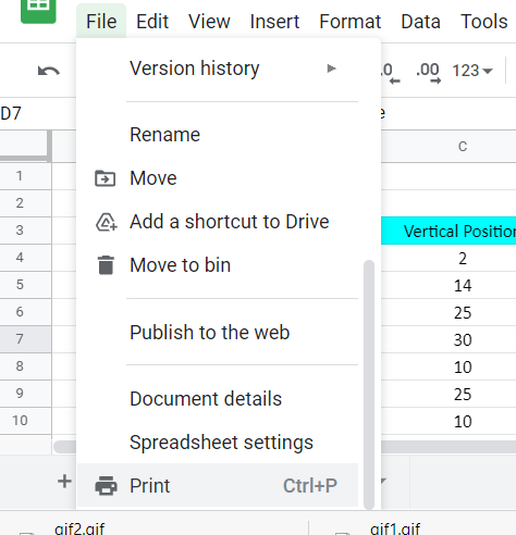
Step 1: Goto File-> Print and Click.
Step 2: Under the Print Settings, in the lower Right Hand Corner , click the check-box of gridlines.
That’s it on this topic. If you face any issues in implementing the above methods then leave a comment down below. Keep browsing SheetsInfo for more such useful information 🙂