At times you may want to hide rows to make your presentation clear and avoid over-burdening of information.
This is very much possible in Google Sheets with the help of easy shortcuts or options. In this tutorial we will go through all the available options to hide or unhide rows in Google Sheet.
Let’s begin.
Table of Contents
Keyboard Shortcut to Hide Rows in Google Sheet
This is probably the easiest of the lot. Follow the below steps:-
- Select any cell(s) in the row(s) which you want to hide
- Now type “CTRL+ALT+9”
The rows will get hidden as expected.

Hiding Rows in Google Sheet using Right Click Option
This approach is most well known and widely used. Follow the below steps:-
- Click on the row numbers you want to hide
- Now Right Click
- Select Hide Rows
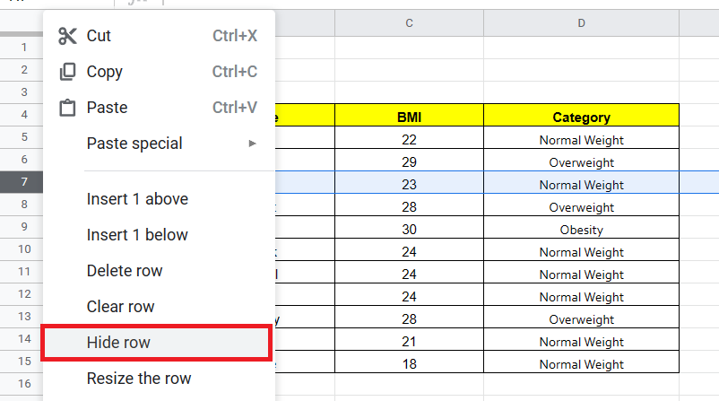
Step 1: Say we want to Hide rows 7. Take your mouse over row number 7 and right click.

Step 2: Click “Hide Row”

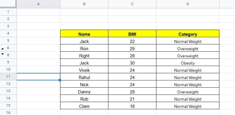
Step 3 : Row 7, gets hidden as expected. Notice the arrows that appear at row 6 & 8 indicating that there’s a hidden row in between.

If you want to hide multiple rows then you need to select multiple rows and perform the same operation. Below is a demo.

Unhiding Rows in Google Sheet
Knowing to Unhide the rows is as important as knowing to hide it.
Here’s a simple hack. All hidden rows come with a two sides arrow symbol.

We simply have to click it to show the hidden rows.

Other way is to simply select the rows around the hidden rows. Right Click and select “Unhide Rows”.

Closing Remarks
As you would have seen this was easy tutorial overall. You might also be interested in showing/hiding columns. If Yes, click the link below to read it.
Show or Hide Columns in Google Sheet
An important call out is that we can hide rows or columns in Google Sheet. However, there is no particular way to hide specific cells in Google Sheet standalone.
That’s it on this topic. If you face any issues in implementing the above methods then leave a comment down below. Keep browsing SheetsInfo for more such useful information 🙂


